
Learning Objectives
Open multiple common remotely sensed image types.
Handle RGB, BGR, LandSat, PlanetScope images, and other sensor types.
Mosaic multiple remotely sensed images.
Create a time series stack.
Write files to disk.
Review
Reading/Writing Remote Sensed Images#
GeoWombat’s file opening is meant to mimic Xarray and Rasterio. That is, rasters are typically opened with a context manager using the function geowombat.open. GeoWombat uses xarray.open_rasterio to load data into an xarray.DataArray. In GeoWombat, the data are always chunked, meaning the data are always loaded as Dask arrays. As with xarray.open_rasterio, the opened DataArrays always have at least 1 band.
Opening a single image#
Opening an image with default settings looks similar to xarray.open_rasterio and rasterio.open. geowombat.open expects a file name (str or pathlib.Path).
import geowombat as gw
from geowombat.data import l8_224078_20200518
import matplotlib.pyplot as plt

with gw.open(l8_224078_20200518) as src:
    print(src)
<xarray.DataArray (band: 3, y: 1860, x: 2041)> Size: 23MB
dask.array<open_rasterio-54cbbadf05c93e93dcee5fb4f30ac048<this-array>, shape=(3, 1860, 2041), dtype=uint16, chunksize=(3, 256, 256), chunktype=numpy.ndarray>
Coordinates:
  * band     (band) int64 24B 1 2 3
  * x        (x) float64 16kB 7.174e+05 7.174e+05 ... 7.785e+05 7.786e+05
  * y        (y) float64 15kB -2.777e+06 -2.777e+06 ... -2.833e+06 -2.833e+06
Attributes: (12/13)
    transform:           (30.0, 0.0, 717345.0, 0.0, -30.0, -2776995.0)
    crs:                 32621
    res:                 (30.0, 30.0)
    is_tiled:            1
    nodatavals:          (nan, nan, nan)
    _FillValue:          nan
    ...                  ...
    offsets:             (0.0, 0.0, 0.0)
    filename:            /home/mmann1123/miniconda3/envs/pygis/lib/python3.11...
    resampling:          nearest
    AREA_OR_POINT:       Area
    _data_are_separate:  0
    _data_are_stacked:   0
In the example above, src is an xarray.DataArray. Thus, printing the object will display the underlying Dask array dimensions and chunks, the DataArray named coordinates, and the DataArray attributes.
It automatically converts the coordinates stored in x and y, and the different bands are stored in band. To select a single band we can simply select it with src.sel(band=1).
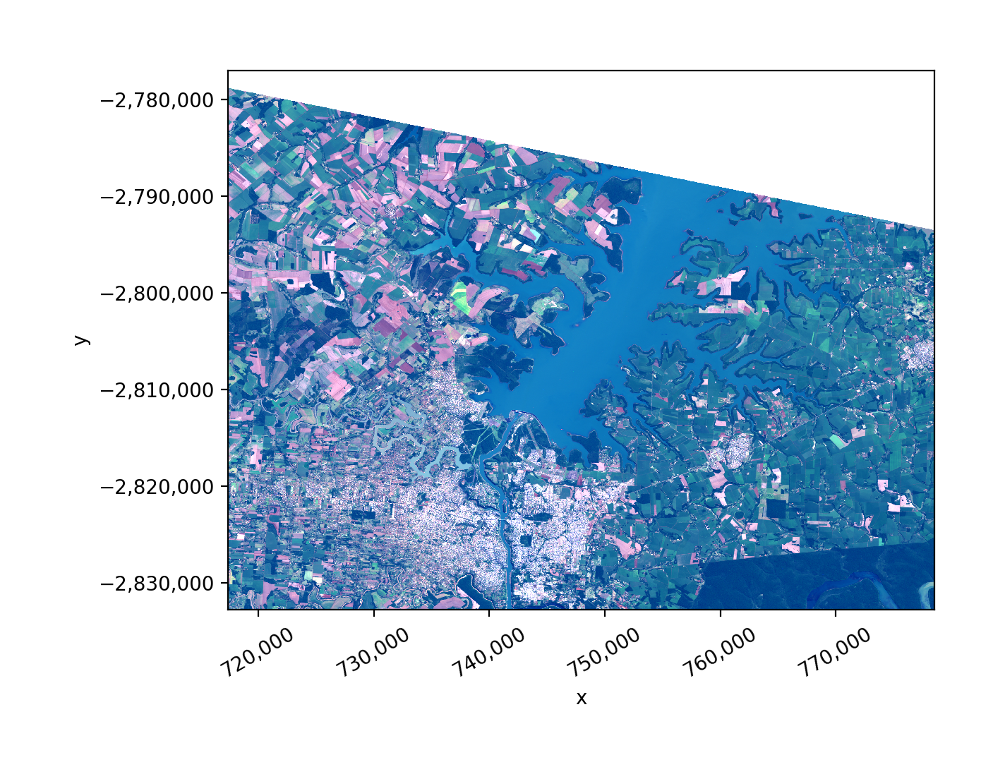
Let’s plot out what we have while removing missing values, stored at 0, and switch the band order around to be RGB.
fig, ax = plt.subplots(dpi=200)
with gw.open(l8_224078_20200518) as src:
    src.where(src != 0).sel(band=[3, 2, 1]).gw.imshow(robust=True, ax=ax)
plt.tight_layout(pad=1)
Opening multiple bands as a stack#
Often, satellite bands will be stored in separate raster files. To open the files as one DataArray, specify a list instead of a file name.
from geowombat.data import l8_224078_20200518_B2, l8_224078_20200518_B3, l8_224078_20200518_B4

with gw.open([l8_224078_20200518_B2, l8_224078_20200518_B3, l8_224078_20200518_B4]) as src:
    print(src)
<xarray.DataArray (time: 3, band: 1, y: 1860, x: 2041)> Size: 23MB
dask.array<concatenate, shape=(3, 1, 1860, 2041), dtype=uint16, chunksize=(1, 1, 256, 256), chunktype=numpy.ndarray>
Coordinates:
  * x        (x) float64 16kB 7.174e+05 7.174e+05 ... 7.785e+05 7.786e+05
  * y        (y) float64 15kB -2.777e+06 -2.777e+06 ... -2.833e+06 -2.833e+06
  * time     (time) int64 24B 1 2 3
  * band     (band) int64 8B 1
Attributes: (12/13)
    transform:           (30.0, 0.0, 717345.0, 0.0, -30.0, -2776995.0)
    crs:                 32621
    res:                 (30.0, 30.0)
    is_tiled:            1
    nodatavals:          (nan,)
    _FillValue:          nan
    ...                  ...
    offsets:             (0.0,)
    filename:            ['LC08_L1TP_224078_20200518_20200518_01_RT_B2.TIF', ...
    resampling:          nearest
    AREA_OR_POINT:       Point
    _data_are_separate:  1
    _data_are_stacked:   1
By default, GeoWombat will stack multiple files by time. So, to stack multiple bands with the same timestamp, change the stack_dim keyword.
Also note the use of band_names parameter. Here we can set it to anything we want for instance ['blue','green','red'].
from geowombat.data import l8_224078_20200518_B2, l8_224078_20200518_B3, l8_224078_20200518_B4

with gw.open(
    [l8_224078_20200518_B2, l8_224078_20200518_B3, l8_224078_20200518_B4],
    stack_dim="band",
    band_names=[1, 2, 3],
) as src:
    print(src)
<xarray.DataArray (band: 3, y: 1860, x: 2041)> Size: 23MB
dask.array<concatenate, shape=(3, 1860, 2041), dtype=uint16, chunksize=(1, 256, 256), chunktype=numpy.ndarray>
Coordinates:
  * x        (x) float64 16kB 7.174e+05 7.174e+05 ... 7.785e+05 7.786e+05
  * y        (y) float64 15kB -2.777e+06 -2.777e+06 ... -2.833e+06 -2.833e+06
  * band     (band) int64 24B 1 2 3
Attributes: (12/13)
    transform:           (30.0, 0.0, 717345.0, 0.0, -30.0, -2776995.0)
    crs:                 32621
    res:                 (30.0, 30.0)
    is_tiled:            1
    nodatavals:          (nan,)
    _FillValue:          nan
    ...                  ...
    offsets:             (0.0,)
    filename:            ['LC08_L1TP_224078_20200518_20200518_01_RT_B2.TIF', ...
    resampling:          nearest
    AREA_OR_POINT:       Point
    _data_are_separate:  1
    _data_are_stacked:   1
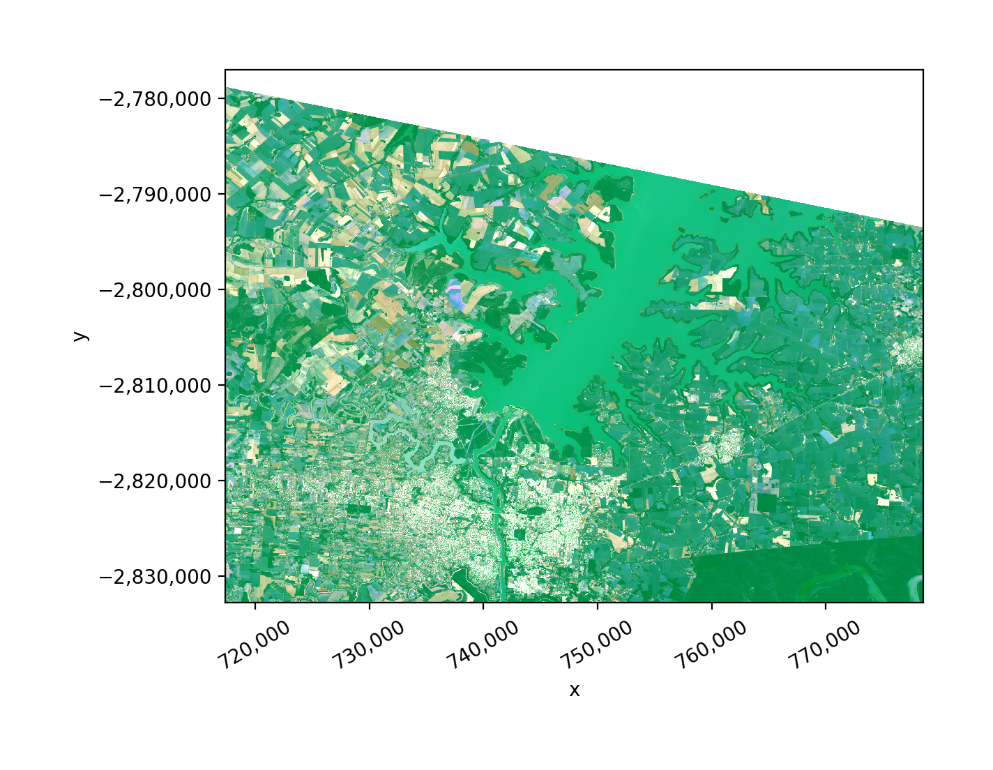
You will see this looks the same as the multiband raster:
fig, ax = plt.subplots(dpi=200)
with gw.open(
    [l8_224078_20200518_B2, l8_224078_20200518_B3, l8_224078_20200518_B4],
    stack_dim="band",
    band_names=['blue','green','red'],
) as src:
    src.where(src != 0).sel(band=['red','blue','green']).gw.imshow(robust=True, ax=ax)
plt.tight_layout(pad=1)
Note
If time names are not specified with stack_dim = ‘time’, GeoWombat will attempt to parse dates from the file names. This could incur significant overhead when the file list is long. Therefore, it is good practice to specify the time names.
Overhead required to parse file names
with gw.open(long_file_list, stack_dim='time') as src:
      ...
No file parsing overhead
with gw.open(long_file_list, time_names=my_time_names, stack_dim='time') as src:
    ...
Opening images from different sensors#
One of many complications of using remotely sensed data is that there are so many different sensors such as LandSat, Sentinel, PlantScope etc each with their own band order and properties. Geowombat makes this much easier by providing a broad list of potential sensor configurations. Read in more detail about sensor configurations here. For this section, let’s keep things simple and show you how to open a Sentinel 2 image using the configuration manager, frankly, it’s pretty easy:
with gw.config.update(sensor='s2'):
    with gw.open('filepath.tif') as src:
        print(src.band)
To see all available sensor names, use the avail_sensors property.
with gw.open('filepath.tif') as src:
    for sensor_name in src.gw.avail_sensors:
        print(sensor_name)
Opening multiple bands as a mosaic#
When a list of files are given, GeoWombat will stack the data by default. To mosaic multiple files into the same band coordinate, use the mosaic keyword.
from geowombat.data import l8_224077_20200518_B2, l8_224078_20200518_B2

with gw.open([l8_224077_20200518_B2, l8_224078_20200518_B2],
              mosaic=True) as src:
    print(src)
<xarray.DataArray '_nanmax_skip-aggregate-02d2d81040a2be2548b7531040edf2d4' (
                                                                             band: 1,
                                                                             y: 1515,
                                                                             x: 2006)> Size: 24MB
dask.array<where, shape=(1, 1515, 2006), dtype=float64, chunksize=(1, 256, 256), chunktype=numpy.ndarray>
Coordinates:
  * band     (band) int64 8B 1
  * x        (x) float64 16kB 6.94e+05 6.94e+05 ... 7.541e+05 7.542e+05
  * y        (y) float64 12kB -2.767e+06 -2.767e+06 ... -2.812e+06 -2.812e+06
Attributes: (12/13)
    scales:              (1.0,)
    offsets:             (0.0,)
    nodatavals:          (nan,)
    _FillValue:          nan
    transform:           (30.0, 0.0, 694005.0, 0.0, -30.0, -2766615.0)
    crs:                 32621
    ...                  ...
    is_tiled:            1
    AREA_OR_POINT:       Point
    resampling:          nearest
    geometries:          [<POLYGON ((754185 -2812065, 754185 -2766615, 694005...
    _data_are_separate:  1
    _data_are_stacked:   0
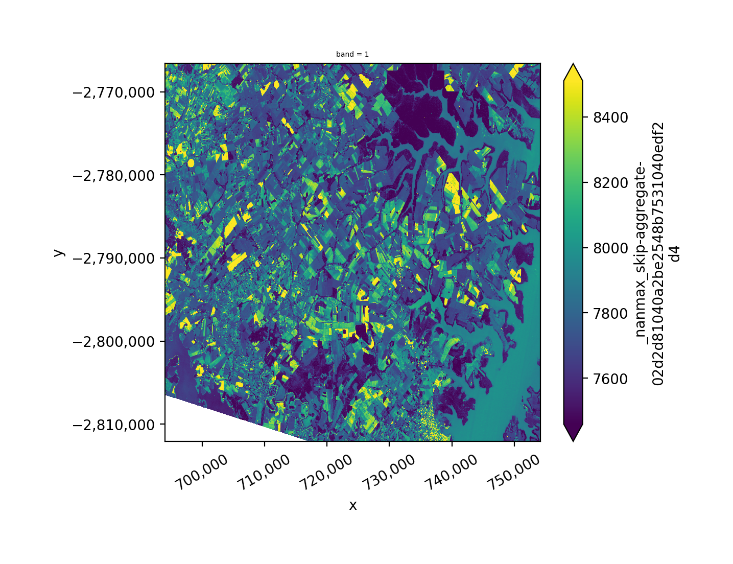
Now let’s take a look at the mosaiced band 2 image values.
fig, ax = plt.subplots(dpi=200)
with gw.open([l8_224077_20200518_B2, l8_224078_20200518_B2],
              mosaic=True) as src:
    src.where(src != 0).sel(band=1).gw.imshow(robust=True, ax=ax)
plt.tight_layout(pad=1)
Create a Time Series Stack#
Let’s pretend for a moment that we have a time series of images from the same tile. We can stack them by passing a list of file names [l8_224078_20200518, l8_224078_20200518], it also helps to be specific and assign time_names=['t1', 't2'], and specify which dimension we want to stack our data along with stack_dim='time'.
with gw.open([l8_224078_20200518, l8_224078_20200518],
            band_names=['blue', 'green', 'red'],
            time_names=['t1', 't2'],
            stack_dim='time') as src:
    print(src)
<xarray.DataArray (time: 2, band: 3, y: 1860, x: 2041)> Size: 46MB
dask.array<concatenate, shape=(2, 3, 1860, 2041), dtype=uint16, chunksize=(1, 3, 256, 256), chunktype=numpy.ndarray>
Coordinates:
  * x        (x) float64 16kB 7.174e+05 7.174e+05 ... 7.785e+05 7.786e+05
  * y        (y) float64 15kB -2.777e+06 -2.777e+06 ... -2.833e+06 -2.833e+06
  * time     (time) <U2 16B 't1' 't2'
  * band     (band) <U5 60B 'blue' 'green' 'red'
Attributes: (12/13)
    transform:           (30.0, 0.0, 717345.0, 0.0, -30.0, -2776995.0)
    crs:                 32621
    res:                 (30.0, 30.0)
    is_tiled:            1
    nodatavals:          (nan, nan, nan)
    _FillValue:          nan
    ...                  ...
    offsets:             (0.0, 0.0, 0.0)
    filename:            ['LC08_L1TP_224078_20200518_20200518_01_RT.TIF', 'LC...
    resampling:          nearest
    AREA_OR_POINT:       Area
    _data_are_separate:  1
    _data_are_stacked:   1
Setting Missing Values#
Many raster files do not have the missing value set properly in their profile. Geowombat makes it easy to set or update the missing data value using nodata in either gw.open or even in gw.config.update if you prefer.
fig, ax = plt.subplots(dpi=200)
with gw.open(l8_224078_20200518, nodata=0) as src:
    # replace 0 with nan
    src = src.gw.mask_nodata()
    src.sel(band=[3, 2, 1]).gw.imshow(robust=True, ax=ax)
plt.tight_layout(pad=1)
Writing DataArrays to file#
The recommended way to write a GeoWombat DataArray to disk is the .gw.save() accessor. It preserves the CRS, transform, and nodata value, handles Dask-backed arrays, and writes in parallel. to_vrt is still available for VRT output. In the examples below, src is an xarray.DataArray with the necessary transform information to write to an image file.
Write to a VRT file.
from geowombat.data import l8_224077_20200518_B4

# Transform the data to lat/lon
with gw.config.update(ref_crs=4326):

    with gw.open(l8_224077_20200518_B4) as src:

        # Write the data to a VRT
        gw.to_vrt(src, 'lat_lon_file.vrt')
Write to a raster file.
import geowombat as gw

with gw.open(l8_224077_20200518_B4) as src:

    # Xarray drops attributes
    attrs = src.attrs.copy()

    # Apply operations on the DataArray
    src = src * 10.0

    src.attrs = attrs

    # Write the data to a GeoTiff — .gw.save() is the default writer
    src.gw.save('output.tif', overwrite=True)