---

Learning Objectives

• Create and manipulate vector attributes

• Subset data

• Plot lat lon as points

• Subset points by location

Review

• Vector Data

---

Attributes & Indexing for Vector Data

Fig. 51 Structure of a GeoDataFrame extends the functionality of a Pandas DataFrame

Each GeoSeries can contain any geometry type (e.g. points, lines, polygon) and has a GeoSeries.crs attribute, which stores information on the projection (CRS stands for Coordinate Reference System). Therefore, each GeoSeries in a GeoDataFrame can be in a different projection, allowing you to have, for example, multiple versions of the same geometry, just in a different CRS.

Tip

Becuase GeoPandas are so intertwined spend the time to learn more about here Pandas User Guide

Create New Attributes

One of the most basic operations is creating new attributes. Let’s say for instance we want to look at the world population in millions. We can start with an existing column of data pop_est. Let’s start by looking at the column names:

import geopandas
world = geopandas.read_file('https://d2ad6b4ur7yvpq.cloudfront.net/naturalearth-3.3.0/ne_50m_admin_0_sovereignty.geojson')
world.columns

Index(['scalerank', 'labelrank', 'sovereignt', 'sov_a3', 'adm0_dif', 'level',
       'type', 'admin', 'adm0_a3', 'geou_dif', 'geounit', 'gu_a3', 'su_dif',
       'subunit', 'su_a3', 'brk_diff', 'name', 'name_long', 'brk_a3',
       'brk_name', 'brk_group', 'abbrev', 'postal', 'formal_en', 'formal_fr',
       'note_adm0', 'note_brk', 'name_sort', 'name_alt', 'mapcolor7',
       'mapcolor8', 'mapcolor9', 'mapcolor13', 'pop_est', 'gdp_md_est',
       'pop_year', 'lastcensus', 'gdp_year', 'economy', 'income_grp',
       'wikipedia', 'fips_10', 'iso_a2', 'iso_a3', 'iso_n3', 'un_a3', 'wb_a2',
       'wb_a3', 'woe_id', 'adm0_a3_is', 'adm0_a3_us', 'adm0_a3_un',
       'adm0_a3_wb', 'continent', 'region_un', 'subregion', 'region_wb',
       'name_len', 'long_len', 'abbrev_len', 'tiny', 'homepart',
       'featureclass', 'geometry'],
      dtype='object')

We can then do basic operations on the basis of column names. Here we create a new column m_pop_est:

world['m_pop_est'] = world['pop_est'] / 1e6
world.head(2)

	scalerank	labelrank	sovereignt	sov_a3	adm0_dif	level	type	admin	adm0_a3	geou_dif	...	subregion	region_wb	name_len	long_len	abbrev_len	tiny	homepart	featureclass	geometry	m_pop_est
0	1	3	Afghanistan	AFG	0	2	Sovereign country	Afghanistan	AFG	0	...	Southern Asia	South Asia	11	11	4	-99	1	Admin-0 sovereignty	POLYGON ((74.89131 37.23164, 74.84023 37.22505...	28.400000
1	1	3	Angola	AGO	0	2	Sovereign country	Angola	AGO	0	...	Middle Africa	Sub-Saharan Africa	6	6	4	-99	1	Admin-0 sovereignty	MULTIPOLYGON (((14.19082 -5.87598, 14.39863 -5...	12.799293

2 rows × 65 columns

---

Indexing and Selecting Data

GeoPandas inherits the standard pandas methods for indexing/selecting data. This includes label based indexing with .loc and integer position based indexing with .iloc, which apply to both GeoSeries and GeoDataFrame objects. For more information on indexing/selecting, see the pandas documentation.

Selection by Index Position

Pandas provides a suite of methods in order to get purely integer based indexing. The semantics follow closely Python and NumPy slicing. These are 0-based indexing. When slicing, the start bound is included, while the upper bound is excluded. For instance name = 'fudge' with name[0:3] returns 'fud', where f is at 0 and g is at the 3 position with the upper bound excluded.

import matplotlib.pyplot as plt
plt.style.use('bmh') # better for plotting geometries vs general plots.

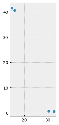
world = geopandas.read_file('https://d2ad6b4ur7yvpq.cloudfront.net/naturalearth-3.3.0/ne_50m_populated_places.geojson')
northern_world = world.iloc[ 0:4 ]    
northern_world.plot(figsize=(10,5))  
plt.show()

Different Choices for Indexing

.loc
.loc is primarily label based, but may also be used with a boolean array. .loc will raise KeyError when the items are not found. Allowed inputs are:

• A single label, e.g. 5 or 'a' (Note that 5 is interpreted as a label of the index. This use is not an integer position along the index.)

• A list or array of labels ['a', 'b', 'c']

• A slice object with labels 'a':'f' (Note that contrary to usual Python slices, both the start and the stop are included, when present in the index! See Slicing with labels and Endpoints are inclusive)

• A boolean array (any NA values will be treated as False)

• A callable function with one argument (the calling Series or DataFrame) and that returns valid output for indexing (one of the above)

See more at Selection by Label.

world.loc[world['NAME'] == 'Singapore']  # Selects the row where the name is 'Singapore'

---

.iloc
.iloc is primarily integer position based (from 0 to length-1 of the axis), but may also be used with a boolean array. .iloc will raise IndexError if a requested indexer is out-of-bounds, except slice indexers which allow out-of-bounds indexing (this conforms with Python/NumPy slice semantics). Allowed inputs are:

• An integer e.g. 5

• A list or array of integers [4, 3, 0]

• A slice object with integers 1:7

• A boolean array (any NA values will be treated as False)

• A callable function with one argument (the calling Series or DataFrame) and that returns valid output for indexing (one of the above)

See more at: Selection by Position and Advanced Indexing.

world.iloc[0]  # Selects the first row  

---

.loc, .iloc, and also [] indexing can accept a callable as indexer.
See more at Selection By Callable.

---

Getting values from an object with multi-axes selection uses the following notation (using .loc as an example, but the following applies to .iloc as well). Any of the axes accessors may be the null slice :. Axes left out of the specification are assumed to be :, e.g. p.loc['a'] is equivalent to p.loc['a', :, :].

Object Type	Indexers
Series	s.loc[indexer]
DataFrame	df.loc[row_indexer,column_indexer]

Subset Points by Location

In addition to the standard pandas methods, GeoPandas also provides coordinate based indexing with the cx indexer, which slices using a bounding box. Geometries in the GeoSeries or GeoDataFrame that intersect the bounding box will be returned.

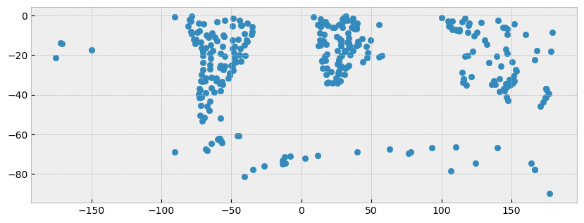
Using the world dataset, we can use this functionality to quickly select all cities in the northern and southern hemisphere using a _CoordinateIndexer using .cx. .cx allows you to quickly access the table’s geometry, where indexing reflects [x,y] or [lon,lat]. Here we will query points above and below 0 degrees latitude:

northern_world = world.cx[ : , 0: ]   # subsets all rows above 0 with a slice
northern_world.plot(figsize=(10, 5))
plt.show()

southern_world = world.cx[ : , :0 ]   # subsets all rows below 0  with a slice
southern_world.plot(figsize=(10, 5))
plt.show()