Setting up a Normal Python Environment

Overview

In this lecture, you will learn how to

1. get a Python environment up and running

2. execute simple Python commands

3. run a sample program

4. install the code libraries that underpin these lectures

Anaconda

The core Python package is easy to install but not what you should choose for these lectures.

These lectures require the entire scientific programming ecosystem, which

• the core installation doesn’t provide

• is painful to install one piece at a time.

Hence the best approach for our purposes is to install a Python distribution that contains

1. the core Python language and

2. compatible versions of the most popular scientific libraries.

The best such distribution is Anaconda.

Anaconda is

• very popular

• cross-platform

• comprehensive

• completely unrelated to the Nicki Minaj song of the same name

Anaconda also comes with a great package management system to organize your code libraries.

Note

All of what follows assumes that you adopt this recommendation!

Installing Anaconda

To install Anaconda, download the binary and follow the instructions.

Important points:

• Install the latest version!

• If you are asked during the installation process whether you’d like to make Anaconda your default Python installation, say yes.

Updating Anaconda

Anaconda supplies a tool called conda to manage and upgrade your Anaconda packages.

One conda command you should execute regularly is the one that updates the whole Anaconda distribution.

As a practice run, please execute the following

1. Open up a terminal

2. Type conda update anaconda

For more information on conda, type conda help in a terminal.

Jupyter Notebooks

Jupyter notebooks are one of the many possible ways to interact with Python and the scientific libraries.

They use a browser-based interface to Python with

• The ability to write and execute Python commands.

• Formatted output in the browser, including tables, figures, animation, etc.

• The option to mix in formatted text and mathematical expressions.

Because of these features, Jupyter is now a major player in the scientific computing ecosystem.

Figure 3 shows the execution of some code (borrowed from here) in a Jupyter notebook

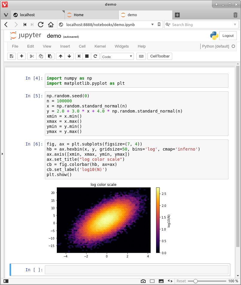
Fig. 3 A Jupyter notebook viewed in the browser

While Jupyter isn’t the only way to code in Python, it’s great for when you wish to

• get started

• test new ideas or interact with small pieces of code

• share scientific ideas with students or colleagues

Starting the Jupyter Notebook

Once you have installed Anaconda, you can start the Jupyter notebook.

Either

• search for Jupyter in your applications menu, or

• open up a terminal and type jupyter notebook

  • Windows users should substitute “Anaconda command prompt” for “terminal” in the previous line.

If you use the second option, you will see something like this

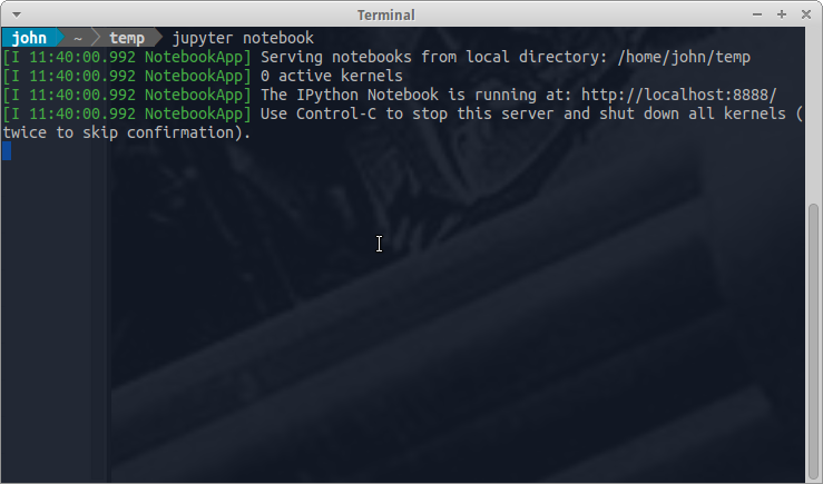
Fig. 4 Terminal window

The output tells us the notebook is running at http://localhost:8888/

• localhost is the name of the local machine

• 8888 refers to port number 8888 on your computer

Thus, the Jupyter kernel is listening for Python commands on port 8888 of our local machine.

Hopefully, your default browser has also opened up with a web page that looks something like this

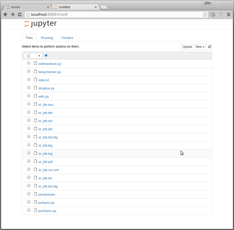
Fig. 5 Jupyter notebook file browser

What you see here is called the Jupyter dashboard.

If you look at the URL at the top, it should be localhost:8888 or similar, matching the message above.

Assuming all this has worked OK, you can now click on New at the top right and select Python 3 or similar.

Here’s what shows up on our machine:

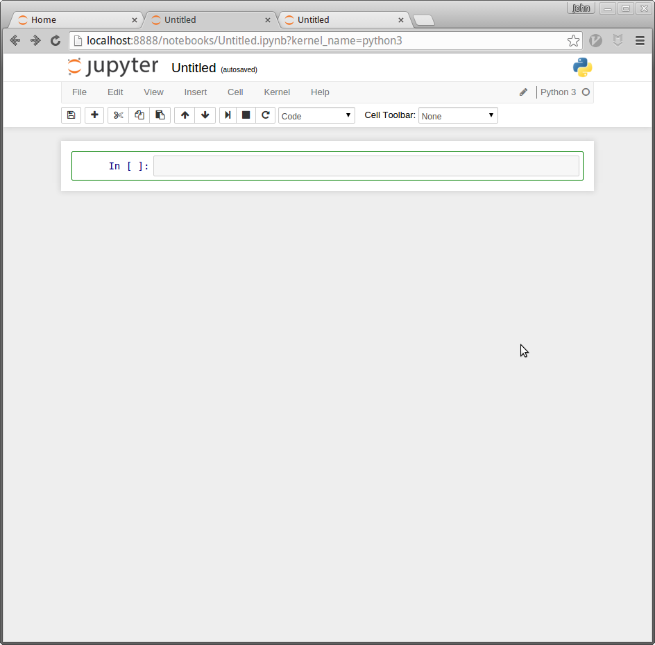
Fig. 6 Jupyter notebook cell

The notebook displays an active cell, into which you can type Python commands.

Notebook Basics

Let’s start with how to edit code and run simple programs.

Running Cells

Notice that, in the previous figure, the cell is surrounded by a green border.

This means that the cell is in edit mode.

In this mode, whatever you type will appear in the cell with the flashing cursor.

When you’re ready to execute the code in a cell, hit Shift-Enter instead of the usual Enter.

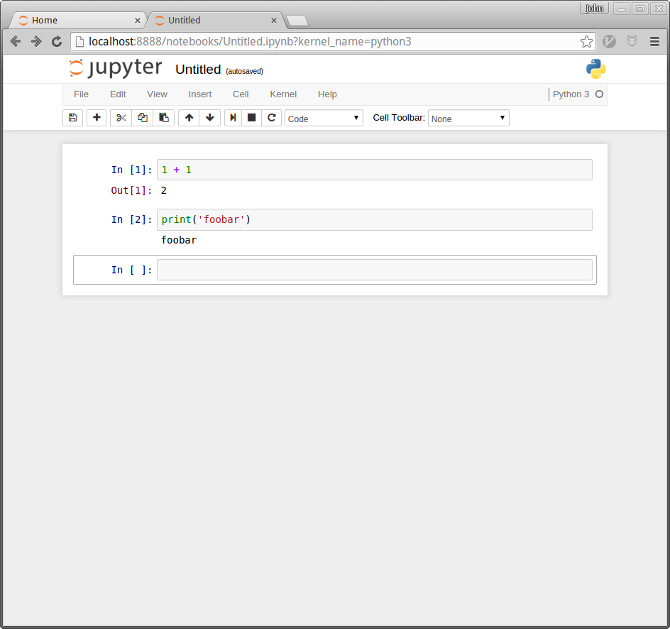
Fig. 7 Running a cell

(Note: There are also menu and button options for running code in a cell that you can find by exploring)

Modal Editing

The next thing to understand about the Jupyter notebook is that it uses a modal editing system.

This means that the effect of typing at the keyboard depends on which mode you are in.

The two modes are

1. Edit mode

   • Indicated by a green border around one cell, plus a blinking cursor

   • Whatever you type appears as is in that cell

2. Command mode

   • The green border is replaced by a grey (or grey and blue) border

   • Keystrokes are interpreted as commands — for example, typing b adds a new cell below the current one

To switch to

• command mode from edit mode, hit the Esc key or Ctrl-M

• edit mode from command mode, hit Enter or click in a cell

The modal behavior of the Jupyter notebook is very efficient when you get used to it.

Inserting Unicode (e.g., Greek Letters)

Python supports unicode, allowing the use of characters such as \(\alpha\) and \(\beta\) as names in your code.

In a code cell, try typing \alpha and then hitting the tab key on your keyboard.

A Test Program

Let’s run a test program.

Here’s an arbitrary program we can use: http://matplotlib.org/3.1.1/gallery/pie_and_polar_charts/polar_bar.html.

On that page, you’ll see the following code

import numpy as np
import matplotlib.pyplot as plt
%matplotlib inline

# Fixing random state for reproducibility
np.random.seed(19680801)

# Compute pie slices
N = 20
θ = np.linspace(0.0, 2 * np.pi, N, endpoint=False)
radii = 10 * np.random.rand(N)
width = np.pi / 4 * np.random.rand(N)
colors = plt.cm.viridis(radii / 10.)

ax = plt.subplot(111, projection='polar')
ax.bar(θ, radii, width=width, bottom=0.0, color=colors, alpha=0.5)

plt.show()

Don’t worry about the details for now — let’s just run it and see what happens.

The easiest way to run this code is to copy and paste it into a cell in the notebook.

Hopefully you will get a similar plot.

Working with the Notebook

Here are a few more tips on working with Jupyter notebooks.

Tab Completion

In the previous program, we executed the line import numpy as np

• NumPy is a numerical library we’ll work with in depth.

After this import command, functions in NumPy can be accessed with np.function_name type syntax.

• For example, try np.random.randn(3).

We can explore these attributes of np using the Tab key.

For example, here we type np.ran and hit Tab

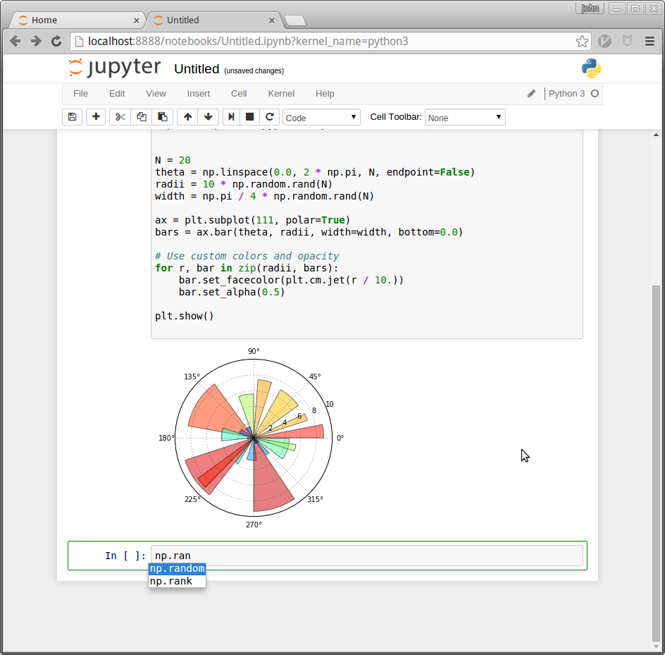
Fig. 8 Tab completion in a notebook

Jupyter offers up the two possible completions, random and rank.

In this way, the Tab key helps remind you of what’s available and also saves you typing.

On-Line Help

To get help on np.rank, say, we can execute np.rank?.

Documentation appears in a split window of the browser, like so

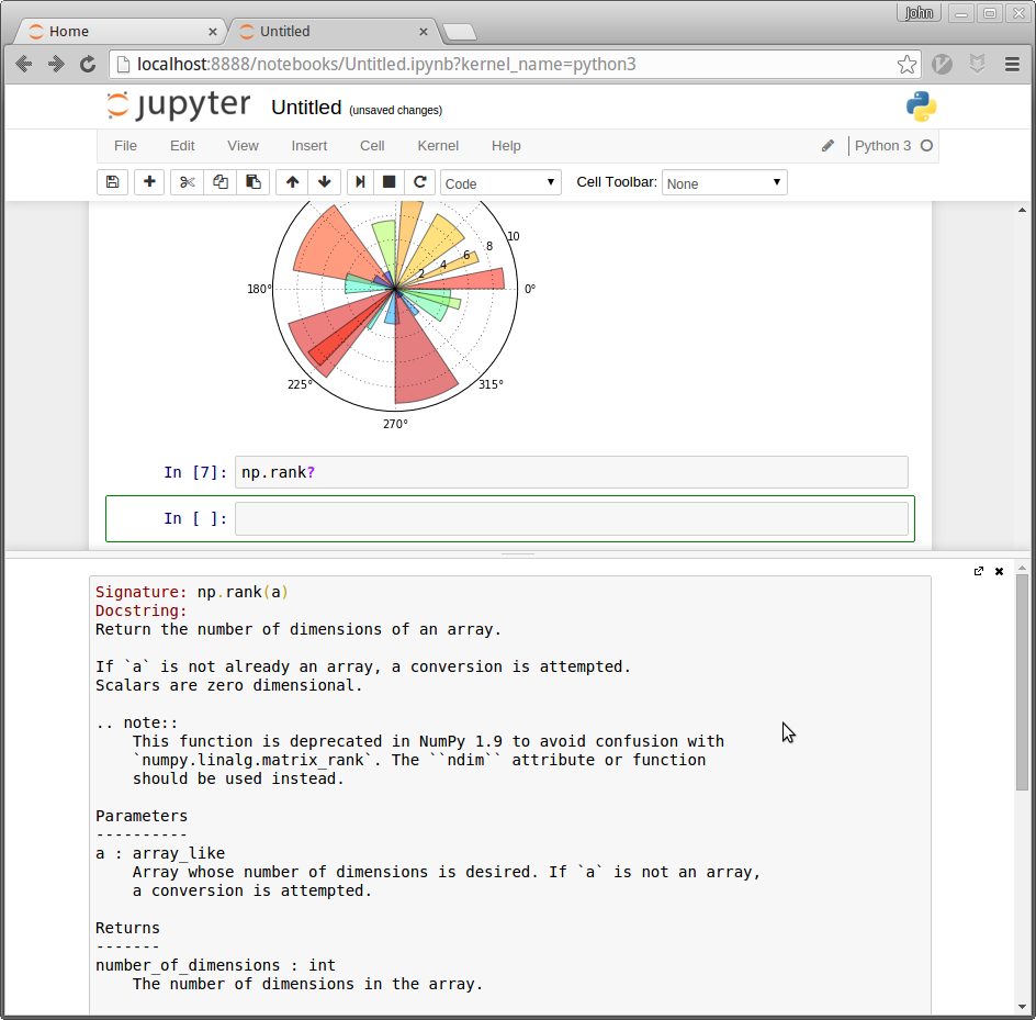
Fig. 9 On-line help in a notebook

Clicking on the top right of the lower split closes the on-line help.

Other Content

In addition to executing code, the Jupyter notebook allows you to embed text, equations, figures and even videos in the page.

For example, here we enter a mixture of plain text and LaTeX instead of code

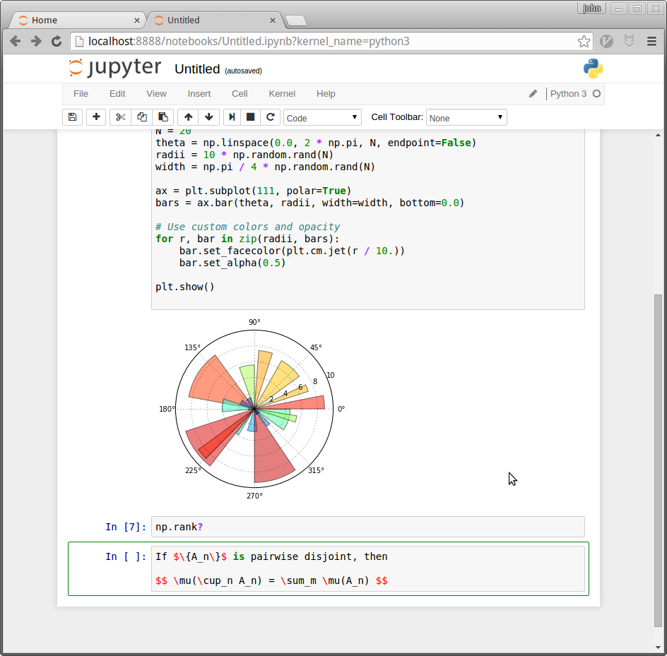
Fig. 10 Markdown in a notebook

Next we Esc to enter command mode and then type m to indicate that we are writing Markdown, a mark-up language similar to (but simpler than) LaTeX.

(You can also use your mouse to select Markdown from the Code drop-down box just below the list of menu items)

Now we Shift+Enter to produce this

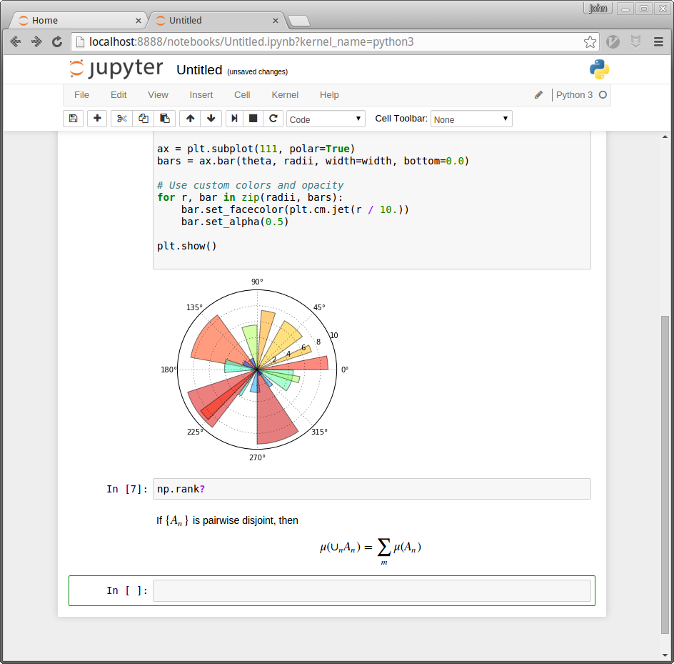
Fig. 11 Markdown rendered in a notebook

Sharing Notebooks

Notebook files are just text files structured in JSON and typically ending with .ipynb.

You can share them in the usual way that you share files — or by using web services such as nbviewer.

The notebooks you see on that site are static html representations.

To run one, download it as an ipynb file by clicking on the download icon.

Save it somewhere, navigate to it from the Jupyter dashboard and then run as discussed above.

Sure! Let’s add a section using Myst Markdown to explain how to access and use Google Colab.

Using Google Colab

Overview

Google Colab is a cloud-based Jupyter notebook environment provided by Google. It allows you to write and execute Python code, similar to Jupyter Notebooks, but without the need for local installations. Google Colab provides free access to computing resources, including GPUs and TPUs, which can be beneficial for resource-intensive tasks.

Accessing Google Colab

To access Google Colab, follow these steps:

1. Open a web browser and navigate to Google Colab.

2. Sign in to your Google account or create one if you don’t have it already.

Creating a New Colab Notebook

Once you are signed in, you can create a new Colab notebook:

1. Click on the “NEW NOTEBOOK” button on the left sidebar or go to “File” > “New notebook.”

Running Code in Colab

Running code in Google Colab is similar to Jupyter Notebooks. You can create code cells and execute them using Shift+Enter or by clicking the “Play” button in the top left of each cell.

print("Hello, Google Colab!")

Hello, Google Colab!

# Basic Python code example
for i in range(5):
    print("Count:", i)

Count: 0
Count: 1
Count: 2
Count: 3
Count: 4

Saving and Sharing Your Colab Notebook

Google Colab automatically saves your notebook in your Google Drive. To save a copy to your local machine or share the notebook with others, go to “File” > “Download” or “File” > “Share.”

GPU and TPU Support

Google Colab provides free access to GPUs and TPUs (Tensor Processing Units) to accelerate computations. To use GPU or TPU, go to “Runtime” > “Change runtime type” and select the desired hardware accelerator.

Accessing External Data

You can access external data from Google Drive, GitHub, or other online sources directly from a Colab notebook. For instance, you can mount your Google Drive and access files using the following code:

from google.colab import drive
drive.mount('/content/drive')

Installing Additional Libraries

Most popular Python libraries come pre-installed in Google Colab. However, if you need to install additional libraries, you can use the pip package manager directly in a code cell:

!pip install pandas

Requirement already satisfied: pandas in /home/mmann1123/miniconda3/envs/pygis2/lib/python3.10/site-packages (1.5.3)

Requirement already satisfied: python-dateutil>=2.8.1 in /home/mmann1123/.local/lib/python3.10/site-packages (from pandas) (2.8.2)
Requirement already satisfied: pytz>=2020.1 in /home/mmann1123/miniconda3/envs/pygis2/lib/python3.10/site-packages (from pandas) (2022.7.1)
Requirement already satisfied: numpy>=1.21.0 in /home/mmann1123/miniconda3/envs/pygis2/lib/python3.10/site-packages (from pandas) (1.24.2)
Requirement already satisfied: six>=1.5 in /home/mmann1123/miniconda3/envs/pygis2/lib/python3.10/site-packages (from python-dateutil>=2.8.1->pandas) (1.16.0)

Limitations

While Google Colab is a powerful tool, it does have some limitations. Colab sessions may disconnect after a period of inactivity, and resources like GPU/TPU availability might be limited during peak usage.

Importantly some libraries used in this textbook, for instance geowombat are not easily installed on google colabs.

Attribution

The above lesson was pulled and adapted from work by Thomas J. Sargent & John Stachurski