---

Learning Objectives

• Learn how rasters are reprojected

• Learn how affine transforms are used

• Use rasterio to reproject a raster

• Learn about interpolation options during transforms

Review

• Intro to Raster data

• Affine transformation

---

Raster Coordinate Reference Systems (CRS)

Raster data is very different that vector data, one of the key differences is that we don’t have a pair of coordinates (x,y) for each pixel in a raster. How then do we know where the raster is located in addition to what the data values are? For a new spatial raster (e.g. geotif) we need to store a few other pieces of information seperately. We need to keep track of the location of the upper left hand corner, the resolution (in both the x and y direction) and a description of the coordinate space (i.e. the CRS), amongst others.

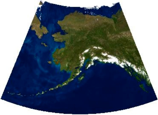
Fig. 42 Example of a warped (reprojected) image

Let’s start from the ndarray Z that we want to span from [-90°,90°] longitude, and [-90°,90°] latitude. For more detail on the construction of these arrays please refer to the raster section.

import numpy as np
import matplotlib.pyplot as plt

x = np.linspace(-90, 90, 6)
y = np.linspace(90, -90, 6)
X, Y = np.meshgrid(x, y)

Z1 =  np.abs(((X - 10) ** 2 + (Y - 10) ** 2) / 1 ** 2)
Z2 =  np.abs(((X + 10) ** 2 + (Y + 10) ** 2) / 2.5 ** 2)
Z =  (Z1 - Z2)

plt.imshow(Z)
plt.title("Temperature")
plt.show()

Note that Z contains no data on its location. Its just an array, the information stored in x and y aren’t associated with it at all. This location data will often be stored in the header of file. In order to ‘locate’ the array on the map we will use affine transformations.

Affine transformations allows us to use simple systems of linear equations to manipulate any point or set of points (review affine transforms here). It allows us to move, stretch, or even rotate a point or set of points. In the case of GIS, it is used to move raster data, a satellite image, to the correct location in the CRS coordinate space.

Describing the Array Location (Define a Projection)

In this example the coordinate reference system will be ‘+proj=latlong’, which describes an equirectangular coordinate reference system with units of decimal degrees. Although X and Y seems relevant to understanding the location of cell values, rasterio instead uses affine transformations instead. Affine transforms uses matrix algebra to describe where a cell is located (translation) and what its resolution is (scale). Review affine transformations and see an example here.

The affine transformation matrix can be computed from the matrix product of a translation (moving N,S,E,W) and a scaling (resolution). First, we start with translation where \(\Delta x\) and \(\Delta y\) define the location of the upper left hand corner of our new Z ndarray. As a reminder the translation matrix takes the form:

\[\begin{split} \begin{eqnarray} \mbox{Translate} = \begin{bmatrix} 1 & 0 & \Delta x \\ 0 & 1 & \Delta y \\ 0 & 0 & 1 \end{bmatrix} \end{eqnarray} \end{split}\]

Now we can define our translation matrix using the point coordinates (x[0],y[0]), but these need to be offset by 1/2 the resolution so that the cell is centered over the coordinate (-90,90). Notice however there are some difference between the x and y resolution:

Both arrays have the same spatial resolution

xres = (x[-1] - x[0]) / len(x)
xres

30.0

But notice that the y resolution is negative:

yres = (y[-1] - y[0]) / len(y)
yres

-30.0

We need to create our translation matrix by defining the location of the upper left hand corner. Looking back at our definitions of our coordinates X and Y we can see that they are defined with x = np.linspace(-90, 90, 6); y = np.linspace(90, -90, 6); X, Y = np.meshgrid(x, y), if you run print(X);print(Y) you will see that the center of the upper left hand corner should be located at (-90,90). The upper left hand corner of that same cell is actually further up and to the left than (-90,90). It follows then that that corner should be shifted exactly 1/2 the resolution of the cell, both up and to the left.

We can therefore define the upper left hand corner by setting \(\Delta x = x[0] - xres / 2\) and \(\Delta y = y[0] - yres / 2\). Remember yres is negative, so subtraction is correct.

from rasterio.transform import Affine
print(Affine.translation(x[0] - xres / 2, y[0] - yres / 2))

| 1.00, 0.00,-105.00|
| 0.00, 1.00, 105.00|
| 0.00, 0.00, 1.00|

We also need to scale our data based on the resolution of each cell, the scale matrix takes the following form:

\[\begin{split} \begin{eqnarray} \mbox{Scale} = \begin{bmatrix} xres & 0 & 0 \\ 0 & yres & 0 \\ 0 & 0 & 1 \end{bmatrix} \end{eqnarray} \end{split}\]

print(Affine.scale(xres, yres))

| 30.00, 0.00, 0.00|
| 0.00,-30.00, 0.00|
| 0.00, 0.00, 1.00|

We can do both operations simultaneously in a new transform matrix by calculating the product of the Translate and Scale matrix:

\[\begin{split} \mbox{Translate} \cdot \mbox{Scale} = \begin{bmatrix} xres & 0 & \Delta x \\ 0 & yres & \Delta y \\ 0 & 0 & 1 \end{bmatrix} \end{split}\]

transform = Affine.translation(x[0] - xres / 2, y[0] - yres / 2) * Affine.scale(xres, yres)
print(transform)

| 30.00, 0.00,-105.00|
| 0.00,-30.00, 105.00|
| 0.00, 0.00, 1.00|

Now we need to write out a tif file that holds the data in Z and its data type with dtype, the location described by transform, in coordinates described by the coordinate reference system +proj=latlon, the number of ‘bands’ of data in count (in this case just one), and the shape in height and width.

import rasterio
with rasterio.open(
    '../temp/Z.tif',
    'w',
    driver='GTiff',
    height=Z.shape[0],
    width=Z.shape[1],
    count=1,
    dtype=Z.dtype,
    crs='+proj=latlong',
    transform=transform,
) as dst:
    dst.write(Z, 1)

All this info is stored in dst and then written to disk with dst.write(Z,1). Where write gets the array of data Z and the band location to write to, in this case band 1. This is a bit awkward, but I believe is a carryover from GDAL which rasterio relies on heavily (like all other platforms including arcmap etc).

The Crazy Tale of the Upper Left Hand Corner

To help us understand what is going on with transform it helps to work an example. For our example above we need to define the translate matrix that helps define the upper left hand corner of our rainfall raster data Z. In particular we need the upper left cell center to be located at (-90,90), so the upper left hand corner need to be 1/2 the resolution above and to the left of (-90,90), implying a location of (-105,105) since the resolution is 30 degrees.

We can visualize what we need to do here:

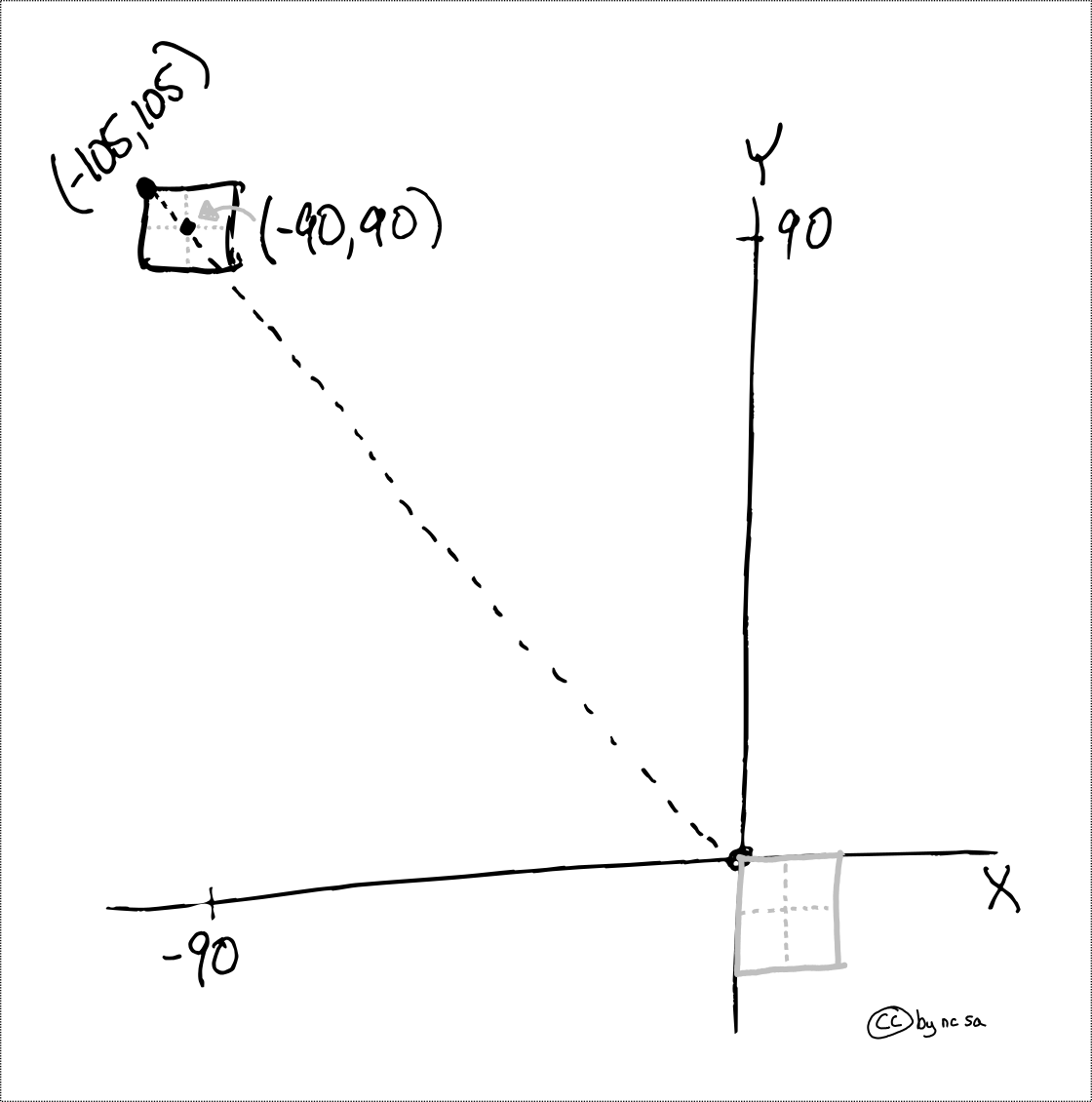
Fig. 43 Example of using translation to shift the upper left hand corner

Let’s walk through the math behind the scenes. Here we use our transform matrix to move our upper left hand corner which is assumed to start at the origin (0,0).

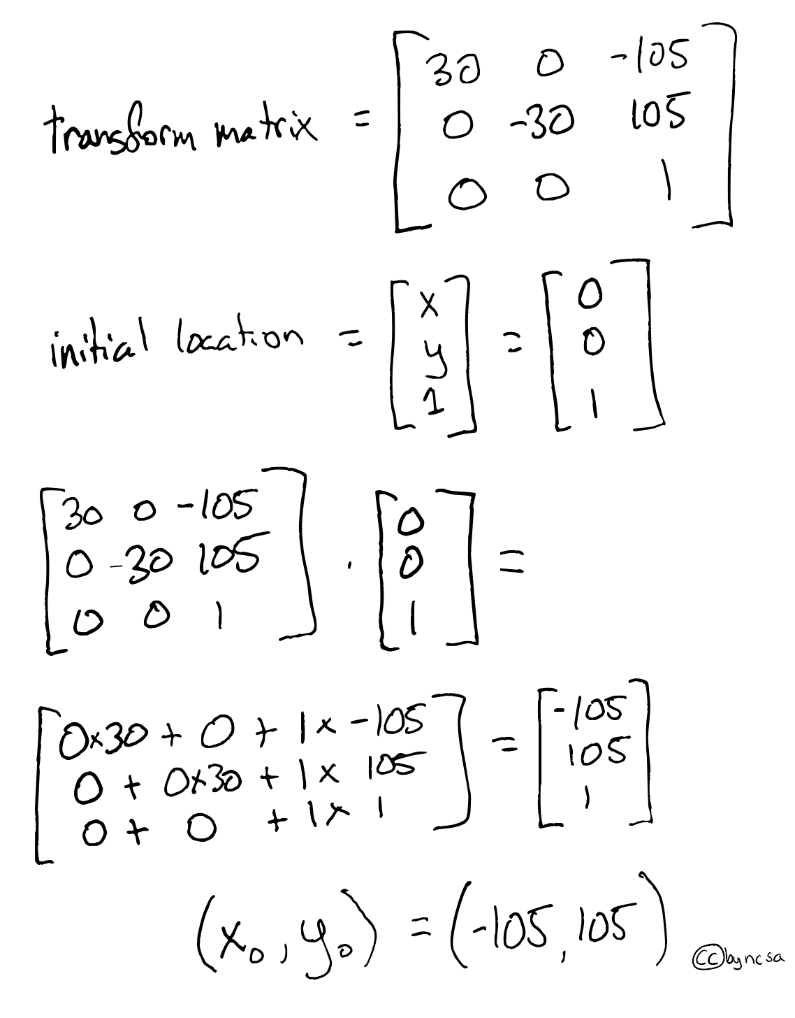
Fig. 44 Example of using affine translation of a matrix to shift the upper left hand corner

The final coordinate of the upper left hand corner are \((x_0,y_0) = (-105,105)\)

Translate is a “map”

Now here’s the magic, our new translate matrix can be used to easily find the coordinates of any cell based on its row and column number. To see how if works, we are going to multiply our translate matrix by (column_number, row_number) to retrieve the coordinates of that cell’s upper right hand corner. Essentially, translate “maps” row and column indexes to coordinates! OMG! This is fun… ok kidding, but it’s useful.

Let’s see how we can calculate a few coordinates (upper left) based on the visual examples below:

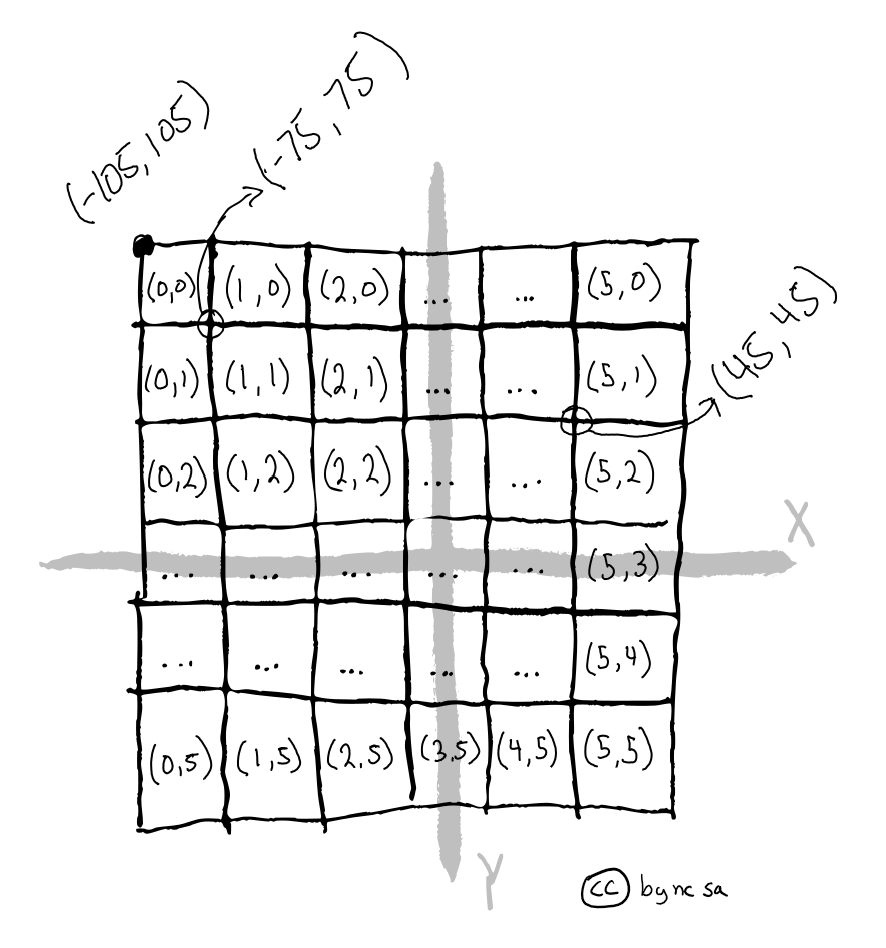
Fig. 45 Example of using transform to identify coordinates based on row and column

Let’s start with the easiest and retrieve the upper left corner coordinates based on transform * (row_number, column_number):

print(transform*(0,0))

(-105.0, 105.0)

Let’s find the corner that is one cell down (-30°) and to the right (+30°)

print(transform*(1,1))

(-75.0, 75.0)

Just to make sure it works let’s find a harder one, 5th column right, 2nd row down:

print(transform*(5,2))

(45.0, 45.0)

How Transforms Works

Let’s work the example of finding the upper left coordinates of with row=5, column=2:

\[\begin{split} \begin{eqnarray} \begin{bmatrix} 30 & 0 & -105 \\ 0 & -30 & 105 \\ 0 & 0 & 1 \end{bmatrix} \begin{bmatrix} 5 \\ 2 \\ 1 \end{bmatrix} = \begin{bmatrix} 5 \times 30 + 2 \times 0 + 1 \times -105 \\ 5 \times 0 + 2 \times -30 + 1 \times 105 \\ 5 \times 0 + 2 \times 0 + 1 \times 1 \end{bmatrix} = \begin{bmatrix} 45 \\ 45 \\ 1 \end{bmatrix} \end{eqnarray} \end{split}\]

Wow, it works! Come on it’s at least a little bit cool. Depending on your definition of cool.

Reproject a Raster - The Simple Case

How then do we reproject a raster? Since transform is a map of pixel locations, warping a raster then becomes as simple as knowing the transform of your destination based on the description of the new coordinate reference system (CRS). If you haven’t please study affine transformations.

Shifting the Prime Meridian

One of the easiest cases is that of false easting, or moving the prime meridian. Let’s walk through an example where we start with a raster with an upper left hand corner at (0, 45), then we will apply a transform to move it to (10, 45) by moving the prime meridian 10° to the west (e.g. using +lon_0=-10 from the proj4string).

Let’s start be looking visually at what we plan to do:

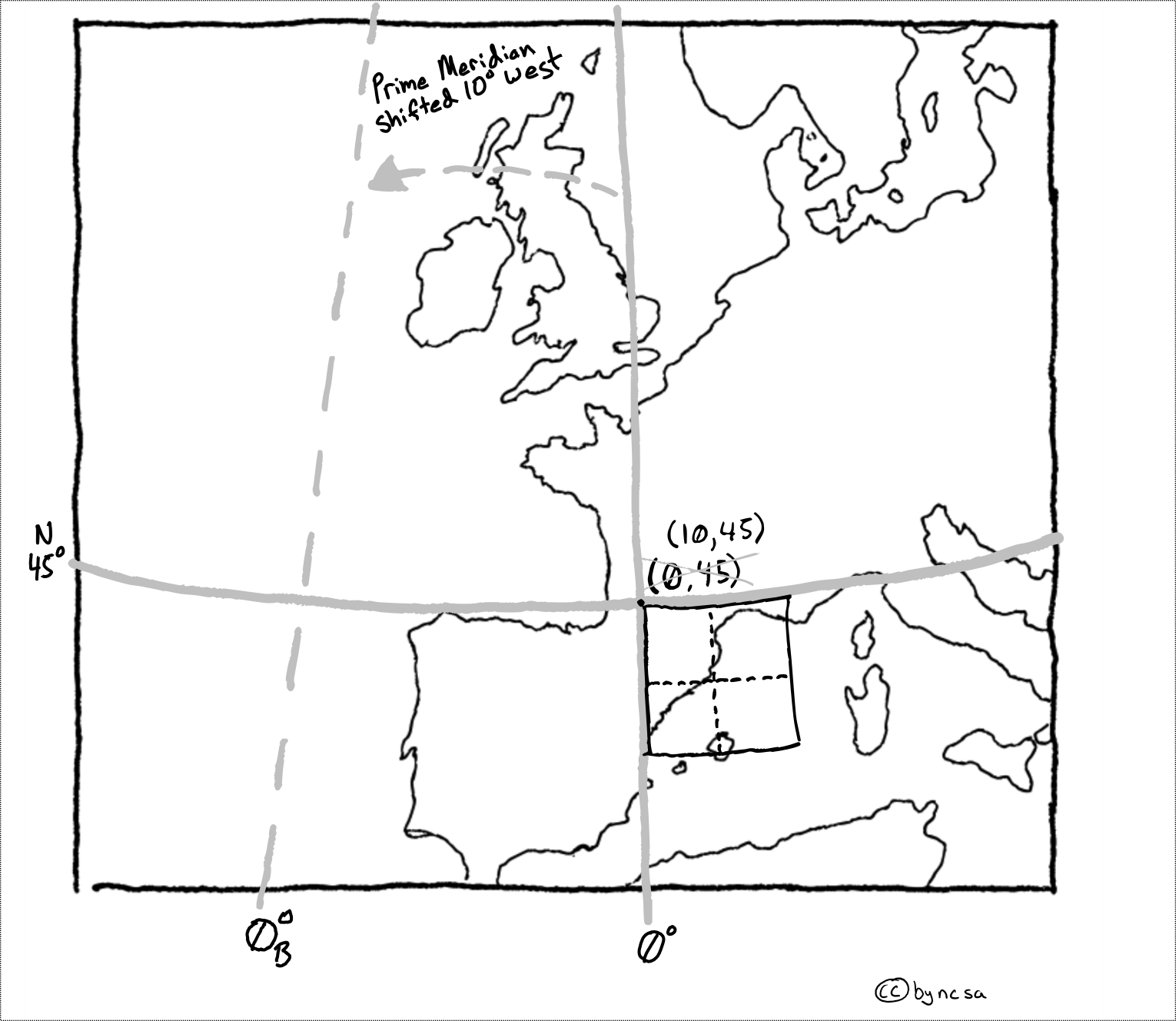
Fig. 46 Example of using translate to reproject an image by moving prime meridian

We can then use our knowledge of matrix algebra and transform matrices to solve for the new upper left hand corner coordinate (\(x_B\), \(y_B\))

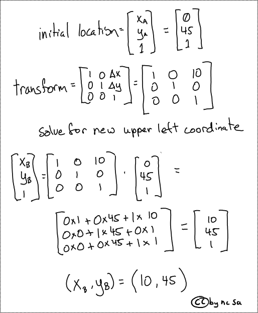
Fig. 47 Example of using translate matrix to reproject an image by moving prime meridian

Reproject a Raster - The Complex Case

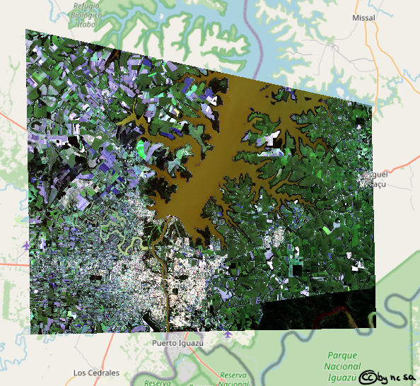
In many cases reprojecting a raster requires changing the number of rows or columns, or ‘warping’ (i.e. bending) an image. All of these examples create a problem, the centroids of the new projected raster don’t line up with the centroids of the original raster. Therefore they now represent locations on the ground that weren’t in the original dataset.

Take for instance the case of a ‘warped’ raster image (below) which for instance occurs when you switch from a spherical CRS (like lat lon) to a projected (or flat) CRS. Notice that the centroids of the two rasters no longer over lap:

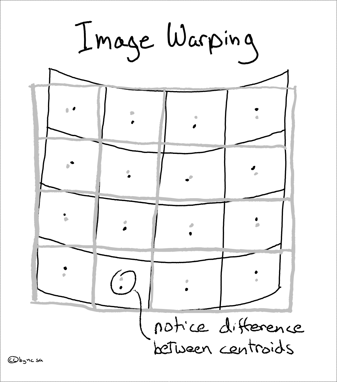
Fig. 48 Example of warping an image during reprojection

In this case we have a decision to make, how will we assign values to the new warped raster? Keep in mind the values must change because they now point to different locations on the ground. For this we have a number of ‘interpolation’ options, some simple, some complex.

Note

What is interpolation? Interpolation allows us to make an informed guess of a value at a new location. Read more here

Interpolation Options

There are three commonly used interpolation methods: a) Nearest neighbor - assigns the value of the nearest centroid, b) bilinear interpolation - uses a straight line between know locations, c) bicubic interpolation - uses curved line between known locations.

In the visual example below we will try to estimate the value for location C based on the known values at locations A and B.

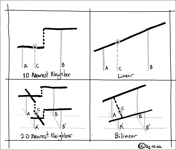
Fig. 49 Example of nearest neighbor and bilinear interpolation

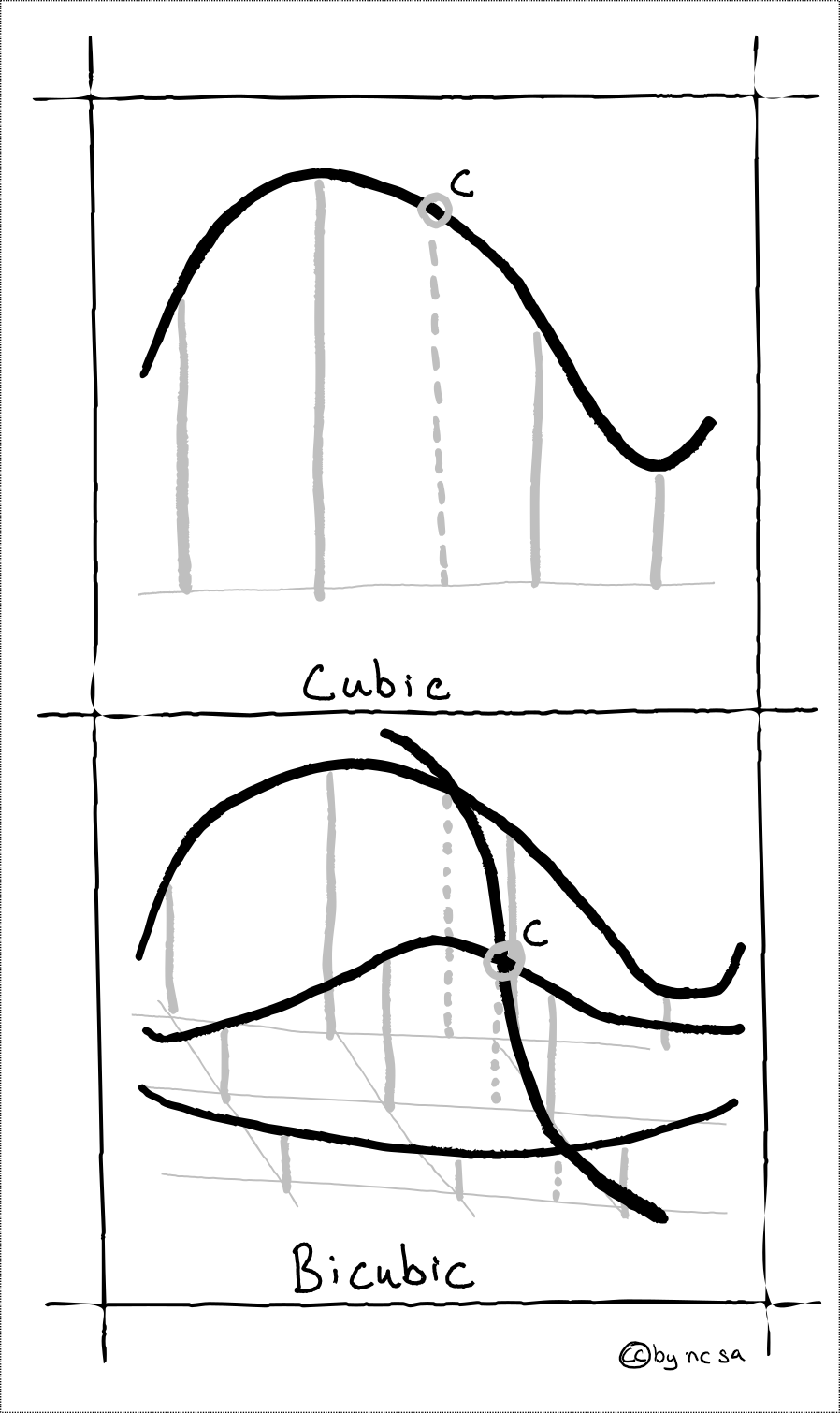
Fig. 50 Example of nearest neighbor and bicubic interpolation

Choosing the Right Interpolation Method

Choosing the correct interpolation method is important. The following table should help you to decided. Remember categorical data might include land cover classes (forest, water, etc), and continuous data is measurable for instance rainfall (values 0 to 20mm).

Method	Description	Fast	Categorical	Continuous
Nearest Neighbor	Assigns nearest value	Y	Y
Bilinear	Linear estimation	Y		Y
Bicubic	Non-Linear estimation	Most of the time		Y

For categorical data, Nearest Neighbor is your only choice, enjoy it. For continuous data, like quantity of rain, you can choose between Bilinear and Bicubic (i.e. “cubic convolution”). For most data Bilinear interpolation is fast and effective. However if you believe your data is highly non-linear, or widely spaced, you might consider using Bicubic. Some experimentation here is often informative.

Reprojecting a Raster with Rasterio

Ok enough talk already, how do we reproject a raster? Before we get into it, we need to talk some more… about calculate_default_transform. calculate_default_transform allows us to generate the transform matrix required for the new reprojected raster based on the characteristics of the original and the desired output CRS. Note that the source (src) is the original input raster, and the destination (dst) is the outputed reprojected raster.

First, remember that the transform matrix takes the following form:

\[\begin{split} \mbox{Transform} = \begin{bmatrix} xres & 0 & \Delta x \\ 0 & yres & \Delta y \\ 0 & 0 & 1 \end{bmatrix} \end{split}\]

Now let’s calculate the tranform matrix for the destination raster:

import numpy as np
import rasterio
from rasterio.warp import reproject, Resampling, calculate_default_transform

dst_crs = "EPSG:3857"  # web mercator(ie google maps)

with rasterio.open("../data/LC08_L1TP_224078_20200518_20200518_01_RT.TIF") as src:

    # transform for input raster
    src_transform = src.transform

    # calculate the transform matrix for the output
    dst_transform, width, height = calculate_default_transform(
        src.crs,    # source CRS
        dst_crs,    # destination CRS
        src.width,    # column count
        src.height,  # row count
        *src.bounds,  # unpacks outer boundaries (left, bottom, right, top)
    )

print("Source Transform:\n",src_transform,'\n')
print("Destination Transform:\n", dst_transform)

Source Transform:
 | 30.00, 0.00, 717345.00|
| 0.00,-30.00,-2776995.00|
| 0.00, 0.00, 1.00| 

Destination Transform:
 | 33.24, 0.00,-6105300.09|
| 0.00,-33.24,-2885952.71|
| 0.00, 0.00, 1.00|

Notice that in order to keep the same number of rows and columns that the resolution of the destination raster increased from 30 meters to 33.24 meters. Also the coordinates of the upper left hand corner have shifted (check \(\Delta x, \Delta x\)).

Ok finally!

dst_crs = "EPSG:3857"  # web mercator(ie google maps)

with rasterio.open("../data/LC08_L1TP_224078_20200518_20200518_01_RT.TIF") as src:
    src_transform = src.transform

    # calculate the transform matrix for the output
    dst_transform, width, height = calculate_default_transform(
        src.crs,
        dst_crs,
        src.width,
        src.height,
        *src.bounds,  # unpacks outer boundaries (left, bottom, right, top)
    )

    # set properties for output
    dst_kwargs = src.meta.copy()
    dst_kwargs.update(
        {
            "crs": dst_crs,
            "transform": dst_transform,
            "width": width,
            "height": height,
            "nodata": 0,  # replace 0 with np.nan
        }
    )

    with rasterio.open("../temp/LC08_20200518_webMC.tif", "w", **dst_kwargs) as dst:
        for i in range(1, src.count + 1):
            reproject(
                source=rasterio.band(src, i),
                destination=rasterio.band(dst, i),
                src_transform=src.transform,
                src_crs=src.crs,
                dst_transform=dst_transform,
                dst_crs=dst_crs,
                resampling=Resampling.nearest,
            )

Fig. 51 Reprojected Landsat Image

Source: Creating Raster Data